Row major order in Data Structure with Example

Row Major Order is a way to represent the elements of a multi-dimensional array in sequential memory. In Row Major Order, elements of a multi-dimensional array are arranged sequentially row by row, which means filling all the index of first row and then moving on to the next row.

C and C++ use Row Major Order by default when storing multi-dimensional arrays.

Important Note: For a 1D array, the concepts of row-major or column-major do not apply since there’s only one dimension.

Visual Example:

Consider storing the elements {1, 2, 3, 4, 5, 6, 7, 8} in a 2×4 array using row-major order.

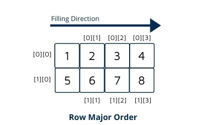
The storage sequence in memory would be: 1, 2, 3, 4, 5, 6, 7, 8 (first row: 1-4, then second row: 5-8). Here first fill index[0][0] and then index[0][1] And for second-row index[1][0] and then index[1][1] and so on..

Row Major Order Formula

The Row Major Order formula calculates the memory address of any element A[i][j] in a 2D array as:

LOC(A[i][j]) = base_address + W * (N * i + j)

Where:

• LOC(A[i][j]): Memory location (address) of element at row i, column j
• base_address: Address of the first element (A[0][0])
• W: Size of each element in bytes (e.g., 4 bytes for int)
• N: Number of columns in the array
• i: Row index (0-based)
• j: Column index (0-based)

Note: This formula assumes 0-based indexing, which is standard in C.

Memory Address Calculation

Problem: Calculate the address of element A[1][2] in a 2×4 integer array with base address 1000. Assume int size is 2 bytes.

Given:

• base_address = 1000
• W = 2 bytes (size of int)
• N = 4 columns
• i = 1 (row index)
• j = 2 (column index)

Solution:

LOC(A[1][2]) = 1000 + 2 × (4 × 1 + 2)
             = 1000 + 2 × (4 + 2)
             = 1000 + 2 × 6
             = 1000 + 12
             = 1012

Therefore, element A[1][2] is stored at memory address 1012.

Row Major Order Examples

1. Two-Dimensional Array (2D)

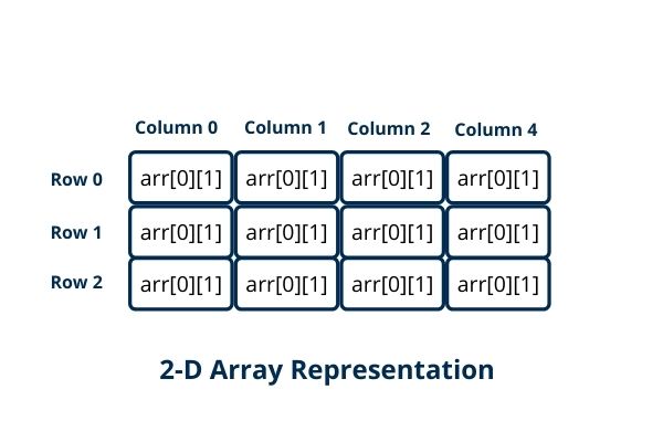
2D Array Declaration in C (2×4 array):

int A[2][4] = {
    {1, 2, 3, 4},    // Row 0
    {5, 6, 7, 8}     // Row 1
};

Logical View (2×4 matrix):

Memory Representation in Row-Major Order:

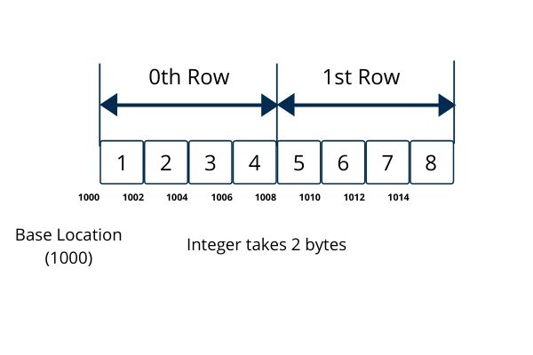
The array is stored in memory as: 1, 2, 3, 4, 5, 6, 7, 8

Corresponding Memory Locations (assuming base address = 1000, int size = 4 bytes):

A[0][0] at address 1000 + 0 = 1000  (value: 1)
A[0][1] at address 1000 + 4 = 1004  (value: 2)
A[0][2] at address 1000 + 8 = 1008  (value: 3)
A[0][3] at address 1000 + 12 = 1012 (value: 4)
A[1][0] at address 1000 + 16 = 1016 (value: 5)
A[1][1] at address 1000 + 20 = 1020 (value: 6)
A[1][2] at address 1000 + 24 = 1024 (value: 7)
A[1][3] at address 1000 + 28 = 1028 (value: 8)

2. Three-Dimensional Array (3D)

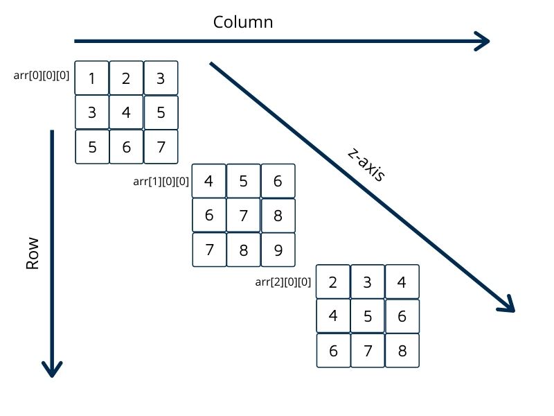
For 3D arrays, row-major order extends naturally: elements are stored layer by layer, and within each layer, row by row.

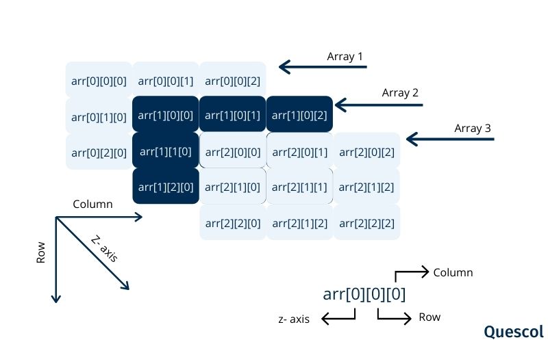
3D Array Declaration in C (3×3×3 array):

int A[3][3][3] = {
    {   // A[0][*][*]
        {1, 2, 3},
        {3, 4, 5},
        {5, 6, 7}
    },
    {   // A[1][*][*]
        {4, 5, 6},
        {6, 7, 8},
        {7, 8, 9}
    },
    {   // A[2][*][*]
        {2, 3, 4},
        {4, 5, 6},
        {6, 7, 8}
    }
};

Memory Storage Sequence (in [k][i][j] format):

A[0][0][0] = 1
A[0][0][1] = 2
A[0][0][2] = 3
A[0][1][0] = 3
A[0][1][1] = 4
A[0][1][2] = 5
A[0][2][0] = 5
A[0][2][1] = 6
A[0][2][2] = 7
A[1][0][0] = 4
A[1][0][1] = 5
A[1][0][2] = 6
A[1][1][0] = 6
A[1][1][1] = 7
A[1][1][2] = 8
A[1][2][0] = 7
A[1][2][1] = 8
A[1][2][2] = 9
A[2][0][0] = 2
A[2][0][1] = 3
A[2][0][2] = 4
A[2][1][0] = 4
A[2][1][1] = 5
A[2][1][2] = 6
A[2][2][0] = 6
A[2][2][1] = 7
A[2][2][2] = 8

General Formula for 3D Arrays

For element A[k][i][j] in an L×M×N array

LOC(A[k][i][j]) = base_address + W × [(M × N × k) + (N × i) + j]

Where k is the first dimension index, i is the second dimension (row) index, and j is the third dimension (column) index.

Key Characteristics of Row-Major Order

• Default in C/C++: Row-major is the default storage scheme for multi-dimensional arrays in C and C++.
• Cache Efficiency: When accessing elements row by row (sequential row access), row-major order provides better cache performance due to spatial locality.
• Rightmost Index Varies Fastest: In the memory sequence, the rightmost index (column index in 2D) changes most frequently.
• Consistent Extension: The concept extends naturally to any number of dimensions (4D, 5D, etc.).
• Contrast with Column-Major: Some languages (like Fortran and MATLAB) use column-major order, where elements are stored column by column.

Practical Implications of Row-Major Order

• Performance Optimization: To maximize cache efficiency in C, iterate through arrays with the rightmost index in the innermost loop:

  // Efficient: Rightmost index 'j' in innermost loop
  for(int i = 0; i < rows; i++) {
      for(int j = 0; j < cols; j++) {
          // Access A[i][j]
      }
  }

• Memory Address Calculation: Understanding row-major order is essential for pointer arithmetic and manual memory management.
• Inter-language Communication: When sharing array data between C (row-major) and Fortran (column-major) programs, transposition may be necessary.