Sparse Matrix and its representation with example

In the world of data structures and mathematical computing, matrices play a crucial role in representing structured data. A matrix is a two-dimensional array consisting of rows and columns, typically denoted as an m × n matrix, where m represents the number of rows and n represents the number of columns.

However, in many real-world applications such as machine learning, image processing, and scientific simulations, most elements in a matrix are often zero. When a matrix contains more zero elements than non-zero elements, it is called a Sparse Matrix.

In contrast to a dense matrix (which contains mostly non-zero values), storing a sparse matrix using traditional two-dimensional arrays is memory-inefficient, as it wastes significant space on zeros. This is where sparse matrix representation becomes valuable. It efficiently stores and processes such matrices by focusing only on the non-zero elements.

What is a Sparse Matrix?

A sparse matrix is a matrix in which most elements are zero. Unlike dense matrices where most elements are non-zero, sparse matrices contain relatively few non-zero entries. They are widely used in fields such as scientific computing, data analysis, network theory, and machine learning.

Key Differences

• Sparse Matrix: Primarily contains zeros
• Dense Matrix: Primarily contains non-zero values

Example of a Sparse Matrix

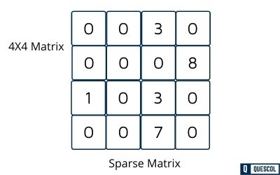
The example above shows a 4×4 matrix where only 5 elements are non-zero, with the remaining 11 elements being zero.

Memory Usage by above Sparse Matrix

Assume each integer occupies 2 bytes of memory, A 4×4 matrix contains 16 elements, requiring:

• Total memory = 16 × 2 = 32 bytes
• Useful memory (for 5 non-zero values) = 5 × 2 = 10 bytes
• Wasted memory = 32 – 10 = 22 bytes (69% waste)

This memory inefficiency escalates dramatically with larger matrices.

Consider a 100×100 matrix with only 10 non-zero elements:

• Traditional storage: 100 × 100 × 2 = 20,000 bytes
• Actual useful data: 10 × 2 = 20 bytes
• Memory wasted: 19,980 bytes (99.9% waste)

Additionally, searching for the 10 non-zero elements would require scanning all 10,000 positions—an extremely inefficient process.

The Problem with Traditional Storage

• Memory Wastage: Significant memory is allocated for zero values that contain no useful information
• Inefficient Processing: Operations must traverse all elements, including zeros, slowing down computations
• Poor Scalability: Memory requirements grow quadratically with matrix size, even with sparse data

The Solution for it is Sparse Matrix Representations

To overcome these limitations, sparse matrix representations store only non-zero elements along with their positions. This approach saves both memory and processing time by ignoring zero elements during storage and operations.

Sparse Matrix Representations

There are two primary methods for representing sparse matrices:

1. Triplet (Coordinate) Representation
2. Linked List Representation

1. Triplet (Coordinate) Representation

In triplet representation, each non-zero element is stored as a triple containing:

• Row index
• Column index
• Value

The first entry (row 0) stores metadata about the original matrix:

• Total number of rows
• Total number of columns
• Total number of non-zero elements

Example: 4×4 matrix with 5 non-zero elements

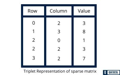
The triplet representation for this matrix would be:

• Row 0: (4, 4, 5) ← Metadata: 4 rows, 4 columns, 5 non-zero elements
• Row 1: (0, 1, 3)
• Row 2: (1, 0, 8)
• Row 3: (2, 2, 1)
• Row 4: (2, 3, 3)
• Row 5: (3, 1, 7)

Benefits of Triplet Representation

• Memory Efficient: Stores only non-zero elements
• Simple Implementation: Easy to understand and implement
• Operation Friendly: Simplifies matrix operations like transpose, addition, and multiplication

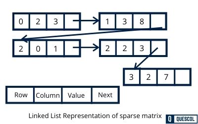
2. Linked List Representation

Linked list representation uses a linked list structure where each node represents one non-zero element. Each node contains four fields:

• Row: Row index of the element
• Column: Column index of the element
• Value: The non-zero value
• Next: Pointer to the next node

Benefits of Linked List Representation

• Dynamic Structure: Easy to insert or delete non-zero elements without reallocating memory
• Memory Efficient: No storage wasted on zero elements
• Scalable: Particularly suitable for matrices where the number of non-zero elements changes frequently

Advantages of Sparse Matrices

• Memory Efficiency: Only non-zero elements are stored, significantly reducing memory requirements
• Faster Processing: Operations only traverse non-zero elements, improving computational speed
• Scalability: Enables working with very large matrices that would be impossible to store in dense format

Sparse Matrix Operations

1. Addition

Adding two sparse matrices involves combining corresponding non-zero elements while preserving the sparse structure.

1. Match Elements: Identify elements with the same (row, column) indices in both matrices
2. Add Matching Values: Sum the values of matching elements
3. Include Unique Elements: Add elements that appear in only one matrix
4. Skip Zeros: Ignore positions where both matrices have zeros

Addition Example

• Matrix A: [(0, 1, 5), (1, 2, 8)]
• Matrix B: [(0, 1, 3), (2, 0, 7)]
• Result C: [(0, 1, 8), (1, 2, 8), (2, 0, 7)]

Note: (0, 1, 8) comes from adding 5 and 3 at position (0,1). Other elements are copied directly from their original matrices.

2. Multiplication

Matrix multiplication of sparse matrices computes dot products while avoiding operations on zero elements.

1. Compute Dot Products: For each row of the first matrix and each column of the second matrix
2. Multiply Matching Elements: Only multiply when column index of first matrix equals row index of second matrix
3. Sum Products: Accumulate products for each result position
4. Skip Zero Operations: Avoid computations involving zero elements

Multiplication Example

• Matrix A (identity): [(0, 0, 1), (1, 1, 1)]
• Matrix B: [(0, 1, 4), (1, 0, 5)]
• Result C: [(0, 1, 4), (1, 0, 5)] (same as B since A is identity)

3. Transpose

Transposition swaps rows and columns while maintaining the sparse structure.

1. Swap Indices: Convert each element from (row, column) to (column, row)
2. Preserve Values: Keep the original element values unchanged
3. Reorganize: Sort elements by their new positions if needed

Transpose Example

• Original A: [(0, 2, 3), (1, 1, 5), (2, 0, 9)]
• Transposed A: [(2, 0, 3), (1, 1, 5), (0, 2, 9)]