Dynamic Programming in Algorithms

Dynamic Programming (DP) is a smart way to solve big problems by breaking them into smaller parts. Many problems contain small subproblems that repeat. Instead of solving the same subproblem again and again, DP solves it once, saves the answer (this is called memoization), and reuses it whenever needed. This saves a lot of time and makes the process faster, just like remembering your homework answers so you do not have to solve the same question again.

Dynamic Programming is widely used in optimization problems, where the goal is to find the most efficient, cost-effective, or fastest solution. Common examples include finding the shortest path, minimizing cost, or maximizing profit. Some Famous DP problems are the Fibonacci sequence, Knapsack problem, and shortest path algorithms in graphs. Overall, Dynamic Programming helps solve problems step by step while using memory wisely to improve speed and efficiency.

Quescol 1-Minute Read

Dynamic Programming (DP) is a method used in computer science to solve complex problems efficiently by breaking them into smaller subproblems that often overlap. It stores the results of these subproblems and reuses them to avoid repeated calculations, making the process faster and more efficient.

This approach significantly improves performance compared to solving each subproblem independently. DP is widely used in optimization problems, where the goal is to find the best, shortest, or most efficient solution.

Key Points of Dynamic Programming

• Core Idea: Solve each subproblem once and store its result for future use.
• Principles: Based on Optimal Substructure and Overlapping Subproblems.
• Approaches:
  • Top-Down (Memoization): Uses recursion and caching.
  • Bottom-Up (Tabulation): Builds the solution iteratively from smaller subproblems.
• Essential Steps:
  1. Understand the problem and define the objective.
  2. Break it into smaller subproblems.
  3. Define the state (what each subproblem represents).
  4. Form the recurrence relation (how states are connected).
  5. Identify base cases.
  6. Choose between top-down or bottom-up approach.
  7. Compute results and extract the final answer.
• Common Examples: Fibonacci Sequence, 0/1 Knapsack, Longest Common Subsequence, Matrix Chain Multiplication, Coin Change, Shortest Path (Bellman-Ford, Floyd-Warshall).

Let’s Understand in Depth

What is Dynamic Programming?

Dynamic Programming (DP) is a problem solving technique that breaks a complex problem into smaller overlapping subproblems, solves each subproblem once, stores the results, and reuses them whenever needed. It avoids the repeated calculations of the same type of problems. This approach reduces computation time and makes the algorithm much faster and more efficient.

Real-Life Example of Dynamic Programming

Imagine you’re cooking a big meal with many dishes. Some dishes need the same ingredients, like chopped onions or boiled rice. Instead of chopping onions or boiling rice again and again for each dish, you do it once, store it, and reuse it whenever needed.

That’s what Dynamic Programming does it solves each small problem once, stores the result, and reuses it for bigger problems. This way, you save time and effort, just like saving your prepped ingredients while cooking!

Key Elements of Dynamic Programming

1. Optimal Substructure

• A problem has optimal substructure if the solution to the whole problem can be built from the solutions to its smaller subproblems.
• Example: In Fibonacci, Fib(5) = Fib(4) + Fib(3), The solution of Fib(5) depends on the solutions of smaller problems Fib(4) and Fib(3).

2. Overlapping Subproblems

• Many small problems are repeated multiple times in the process.
• Example: Calculating Fib(5) requires computing Fib(3) more than once. DP solves it a single time and stores the result.

3. Memoization (Top-Down Approach)

• Memoization uses recursion to solve the problem from top to bottom, stores results of computed subproblems so they can be reused later.
• Example: Recursive Fibonacci that uses a table or array to store previously calculated values.

4. Tabulation (Bottom-Up Approach)

• This approach solves the smallest subproblems first and stores their answers in a DP table (usually an array or a 2D table). Then it fills this table step by step using previously stored values until the final answer is reached.
• Example: Start with Fib(0) and Fib(1), then compute Fib(2), Fib(3), and so on until Fib(n).

5. State Definition

• Define how to represent each subproblem, usually using variables or indices. Each state must uniquely describe a subproblem.
• Example: In 0/1 Knapsack, the state is dp[i][w], meaning the maximum value using the first i items with a total allowed weight w.

6. Recurrence / Transition Formula

• This formula describes how to compute a state based on the results of smaller states.
• Example (0/1 Knapsack):
  dp[i][w] = max(dp[i-1][w], value[i] + dp[i-1][w-weight[i]])

7. Base Cases

• These are the smallest or simplest subproblems with already known results.
• Example: Fib(0) = 0, Fib(1) = 1

8. Decision Making

• At each step, DP often requires to decide the best option among multiple choices.
• Example: In Knapsack, the choice is whether to include the current item or skip it.

Steps to Solve a Problem using DP

1. Understand the Problem Clearly

Before solving, make sure you completely understand what the problem is asking. Identify whether it is about maximizing, minimizing, counting, or finding a specific arrangement.

For example, if the problem asks, “Find the maximum value that fits in a knapsack,” you know it’s an optimization problem. Understanding the goal clearly helps you decide how to break it into smaller parts.

2. Break the Problem into Smaller Subproblems

Think about how the big problem can be divided into smaller problems. DP works because solving small problems helps solve the bigger one.

For example, in the Fibonacci sequence, Fib(5) can be broken down into Fib(4) and Fib(3). Breaking the problem helps you see patterns and repetitive calculations.

3. Check for Overlapping Subproblems

See if the same subproblem is calculated more than once. If yes, DP can save time by storing results.

For example, in Fibonacci, Fib(3) is used multiple times. By saving it after the first calculation, you avoid repeating work. Overlapping subproblems are what make DP efficient.

4. Define the State

A “state” is a way to describe a subproblem completely. It should include all the information needed to solve it.

For example, in 0/1 Knapsack, the state can be dp[i][w], representing the maximum value possible using the first i items with weight limit w. Defining states clearly is crucial for building the DP solution.

5. Write the Transition Formula (Recurrence Relation)

Figure out how to go from smaller subproblems to bigger ones. This is your main formula.

For example, in Fibonacci, Fib(n) = Fib(n-1) + Fib(n-2) shows how bigger values depend on smaller ones. The transition formula is the key to connecting all subproblems together.

6. Set Base Cases

Identify the simplest problems that have known answers. Base cases act as a starting point for computation.

For example, in Fibonacci, Fib(0) = 0 and Fib(1) = 1. Without base cases, recursion or iteration won’t work correctly.

7. Choose Top-Down or Bottom-Up Approach

Decide whether to use top-down (memoization) or bottom-up (tabulation). Top-down means solving recursively and storing results to reuse. Bottom-up means solving smaller problems first and building up to the bigger problem iteratively. Both approaches use the same states and formulas but differ in the order of computation.

8. Compute Results Step by Step

Now start filling your DP table or memoization structure using your transition formula and base cases. Solve problems in a logical order to ensure all smaller subproblems are solved before using them in bigger ones. For example, in Knapsack, fill the table for all items and all weight limits gradually.

9. Return the Final Answer

After solving all subproblems, the final solution is ready. It is usually stored in the last cell of the DP table or returned from the top-down function. For example, dp[n] in Fibonacci or dp[n][W] in Knapsack gives the answer.

Two Main Approaches of Dynamic Programming

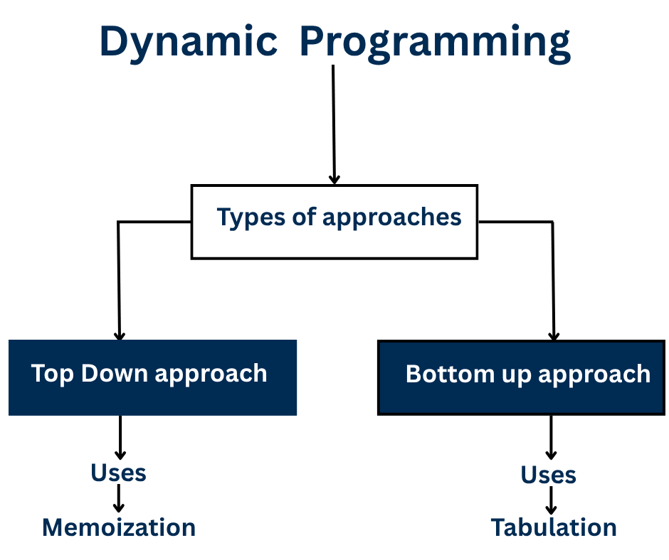
1. Top-Down (Memoization)

The Top Down (Memoization) approach starts with the main problem and breaks it into smaller subproblems only when needed. It uses recursion to move down step by step until it reaches the base cases (the smallest problems). Whenever a subproblem is solved, its answer is stored in memory (such as an array or dictionary). If the same subproblem appears again, the stored answer is reused instead of solving it again. This avoids repeated work and makes the algorithm much faster.

Example of Top-Down

Find Fib(5)

Top down starts from the big problem:

Fib(5)
 ├── Fib(4)
 │     ├── Fib(3)
 │     └── Fib(2)
 └── Fib(3)   ← repeated subproblem

What happens:

• First we ask for Fib(5).
• It needs Fib(4) and Fib(3).
• To find Fib(4), we need Fib(3) and Fib(2).
• But Fib(3) is needed again later — so when we compute it once, we store it.
• Next time Fib(3) is needed, we reuse the stored answer.

Solve only when needed → store → reuse.

2. Bottom-Up (Tabulation)

The Bottom Up (Tabulation) approach works opposite to memoization. Instead of starting with the main problem, it begins by solving the smallest subproblems first and then gradually builds solutions for larger ones. It uses a table or array to store answers for all smaller problems and fills this table step by step until it reaches the final answer. This method does not use recursion — everything is done using loops. It’s like climbing stairs: you start from the bottom step and move up one step at a time until you reach the top.

Example of Bottom-Up

Find Fib(5)

Bottom up starts from the smallest values:

Fib(0) = 0
Fib(1) = 1

Then fill the table step by step:

Fib(2) = 1
Fib(3) = 2
Fib(4) = 3
Fib(5) = 5

What happens:

• We already know Fib(0) and Fib(1).
• Using them, calculate Fib(2).
• Using Fib(1) and Fib(2), calculate Fib(3).
• Continue until Fib(5).

Start from the bottom → build step by step → reach the final answer.

Usages of Dynamic Programming

Below are the list of Problems that we solve using Dynamic Programming.

Problem Name	Description	Example
Fibonacci Sequence	Find nth number in Fibonacci series	F(n) = F(n−1) + F(n−2)
Knapsack Problem	Maximize profit with limited weight	Choose best items for bag
Longest Common Subsequence	Find longest sequence common to two strings	“ABC” & “ACD” → “AC”
Matrix Chain Multiplication	Find minimum multiplications to multiply matrices	Optimize matrix order
Coin Change Problem	Find minimum coins to make certain amount	Amount = 11, coins = [1,2,5]
Shortest Path (Bellman-Ford, Floyd-Warshall)	Find shortest distance between nodes	Network routing
Edit Distance	Find minimum edits to convert one string to another	“CAT” → “CUT” needs 1 change

Fibonacci Problem Example : Without DP and With DP

Without DP (recursive)

int fib(int n) {
    if (n <= 1)
        return n;
    return fib(n-1) + fib(n-2);
}

In this method, the function keeps calling itself again and again to find the Fibonacci number. For every number n, it calls fib(n-1) and fib(n-2) separately. This means the same values are calculated many times, which wastes a lot of time. As n gets bigger, the number of calls grows very fast, almost like doubling each time.

That’s why the time complexity is O(2ⁿ), which makes this method very slow for large n.

With DP (bottom-up)

int fib(int n) {
    int dp[] = new int[n+1];
    dp[0] = 0;
    dp[1] = 1;
    for (int i = 2; i <= n; i++)
        dp[i] = dp[i-1] + dp[i-2];
    return dp[n];
}

In the bottom-up Dynamic Programming approach, we iteratively build the Fibonacci sequence from smaller subproblems. An array dp[] is used to store already computed values, where each dp[i] represents the i-th Fibonacci number. Starting with the base cases dp[0] = 0 and dp[1] = 1, we compute each next value using the relation dp[i] = dp[i-1] + dp[i-2].

This avoids redundant recursive calls and overlapping computations. Since each state is computed exactly once, the time complexity is O(n) and the space complexity is O(n), making it far more efficient than the exponential recursive solution.

Advantages of Dynamic Programming

• Reduces Time Complexity – Avoids recalculating same results again and again: DP stores results of small subproblems, so repeated calculations are avoided. For example, Fibonacci numbers can be computed much faster using DP than plain recursion.
• Efficient for Overlapping Problems – Perfect for recursive problems like Fibonacci, Knapsack, etc.: Problems with repeated subproblems are solved efficiently since each small problem is computed only once and reused.
• Guaranteed Optimal Solution – Always gives the best (optimal) solution: DP keeps track of the best solution at every step, ensuring the final answer is always optimal, like getting maximum profit in Knapsack.
• Can be used in many areas – AI, scheduling, optimization, networking, pathfinding, etc.: DP applies wherever problems can be broken into smaller overlapping parts, such as in AI, task scheduling, network routing, logistics, and bio-informatics. Reduces Time Complexity – Avoids recalculating same results again and again: DP stores results of small subproblems, so repeated calculations are avoided. For example, Fibonacci numbers can be computed much faster using DP than plain recursion.
• Efficient for Overlapping Problems – Perfect for recursive problems like Fibonacci, Knapsack, etc.: Problems with repeated subproblems are solved efficiently since each small problem is computed only once and reused.
• Guaranteed Optimal Solution – Always gives the best (optimal) solution: DP keeps track of the best solution at every step, ensuring the final answer is always optimal, like getting maximum profit in Knapsack.
• Can be used in many areas – AI, scheduling, optimization, networking, pathfinding, etc.: DP applies wherever problems can be broken into smaller overlapping parts, such as in AI, task scheduling, network routing, logistics, and bioinformatics.

Disadvantages of Dynamic Programming

• High Memory Usage – Dynamic Programming needs extra space to store results of subproblems, usually in tables or arrays. This can be significant for very large problems.
• Difficult to Design – DP requires careful analysis to identify the subproblems and how they relate to each other. Designing the right recurrence and storage strategy can be challenging.
• Not for all problems – DP only works for problems that have overlapping subproblems and an optimal substructure. Problems without these properties cannot benefit from DP.
• Debugging Complexity – Since DP involves multiple states and transitions, debugging errors in the recurrence relation or state transitions can be complicated.
• Time Overhead – Even though DP avoids re-computation, it may still take significant time due to large table sizes or high-dimensional states.
• Initialization Issues – Choosing the right base cases and initializing the DP table correctly is often tricky and can lead to wrong results if done incorrectly.
• Difficult to Visualize – For complex problems, understanding how subproblems depend on each other and how states evolve can be hard to conceptualize.
• Limited Scalability – In problems with multiple dimensions (e.g., 3D DP), both time and space complexity can grow exponentially, making them impractical for large inputs.
• Implementation Complexity – Converting a recursive relation into an iterative or memoized version can be error-prone and requires careful thought.

Conclusion

Dynamic Programming (DP) is an efficient method for solving complex problems by breaking them into smaller overlapping subproblems. It stores the solutions of these subproblems to avoid redundant computations and thus improves the overall efficiency of the algorithm.

It is based on two main principles: optimal substructure and overlapping subproblems. By using these principles, DP provides faster and more optimal solutions to problems such as shortest path, knapsack, and sequence alignment.