Travelling Salesman Problem (TSP) Using Branch and Bound

The Travelling Salesman Problem (TSP) is a classical problem in computer science and operations research. It involves finding the shortest possible route for a salesman to visit each city exactly once and return to the starting city. The problem becomes computationally difficult as the number of cities increases, since the number of possible routes grows exponentially, making exhaustive search impractical.

The Branch and Bound technique is an efficient method to solve TSP. In this approach, the problem is systematically divided into smaller sub-problems (branching), and paths that cannot yield a better solution than the current best are eliminated (bounding). By exploring only the promising routes, Branch and Bound reduces unnecessary computations and helps determine the optimal route efficiently.

Quescol 1-Minute Read

The Branch and Bound method is an efficient way to solve the 0/1 Knapsack problem, where we must choose items to maximize value without going over the weight limit. Instead of checking every possible combination like brute force, it breaks the problem into smaller parts (branches) and uses limits (bounds) to skip unnecessary calculations.

It works by exploring a state space tree, where each node represents a decision, whether to include or exclude an item. If a branch can’t lead to a better solution than the best one found so far, that branch is cut off (called pruning). This makes it much faster and more efficient.

Key Points about Travelling Salesman Problem

• Selects items to get the maximum total value without exceeding weight.
• Uses bounding to skip unpromising branches.
• Works with a state space tree.
• Much faster than brute force.
• Always gives the optimal solution.
• Time complexity: O(2ⁿ) in the worst case, but much less in practice due to pruning.
• Space complexity: O(n) (for storing items and tree nodes).

Let’s Understand in Depth

What is Branch and Bound Approach?

The Branch and Bound algorithm is an efficient technique to solve the Travelling Salesman Problem (TSP) without checking every possible route. Instead of checking every possible route (which grows factorially), it reduces the search space by exploring only the most promising paths. It does this through three key steps: branch, bound, and prune.

It works in three main steps:

1. Branch: The algorithm breaks the main problem into smaller subproblems by making choices at each step, such as deciding the next city to visit. This creates a tree of possible routes.
2. Bound: For each subproblem, a lower bound is calculated, which is the minimum possible cost to complete the tour from that point. This helps estimate whether a partial route could lead to an optimal solution.
3. Prune: Any subproblem whose lower bound is higher than the best solution found so far is discarded. This prevents exploring routes that cannot improve the current best solution.

Representation of the TSP Problem in Branch and Bound Approach

To apply Branch and Bound in solving Travelling Salesman Problem (TSP), we first represent the cities and distances as a cost matrix.

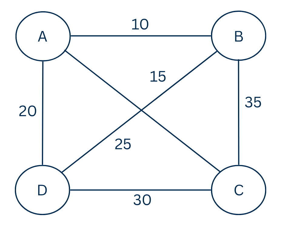
Example: Suppose there are 4 cities (A, B, C, D)

i \ j	A	B	C	D
A	∞	10	15	20
B	10	∞	35	25
C	15	35	∞	30
D	20	25	30	∞

• Each cell (i, j) shows how much it costs to travel from city i to city j.
• If the value is ∞ (infinity), it means that a city cannot travel to itself, for example, going from city A to A is not possible.

Steps to solve TSP Problem using Branch and Bound Algorithm

1. Initialization

• Start from the first city (can be any city).
• Set current minimum cost to a large number (infinity).
• Create a priority queue to store partial solutions (nodes).

2. Node Representation

Each node represents:

• The path so far (cities visited).
• The cost of the path so far.
• The lower bound of total cost if we continue this path.

3. Calculate Lower Bound

The lower bound helps decide whether to continue exploring a path.

How to calculate lower bound for a node:

1. Take the cost so far.
2. Add the minimum possible cost for each unvisited city to complete the tour.

This gives the minimum possible total cost for that partial path.

4. Branching Process

From the current city, create child nodes for each unvisited city.

For each child node:

• Add the new city to the path.
• Update the cost by adding the cost from current city to the new city.
• Calculate the lower bound.

5. Pruning Step

Compare the lower bound of a child node with the current best solution:

• If lower bound >= current minimum cost, discard this node (prune it).
• Otherwise, keep exploring this node.

This ensures we only explore promising paths.

6. Selection of Node

• Always select the node with the smallest lower bound from the priority queue next.
• This is similar to a best-first search strategy.

7. Repeat Until Completion

Repeat branching and pruning until all nodes are either:

• Explored, or
• Pruned

When a complete tour is found (visiting all cities and returning to start), compare its cost with current minimum cost.

Update current minimum cost if this tour is cheaper.

8. Termination

• When there are no more nodes left to explore in the queue, the current minimum cost is the optimal solution.
• The corresponding path is the best route for TSP.

Example Walkthrough (Simple 3-City Example)

Let’s solve this problem for better understanding of TSP using Branch and Bound.

Suppose cities: A, B, C, D
Cost Matrix:

i \ j	A	B	C	D
A	∞	10	15	20
B	10	∞	35	25
C	15	35	∞	30
D	20	25	30	∞

Step 1: Start at A → path A, cost = 0

Step 2: Branch to B, C, D

• Branch to B → A,B, cost = 10
• Branch to C → A,C, cost = 15
• Branch to D → A,D, cost = 20

Step 3: Explore the node with smallest cost first → A,B(cost 10)

Step 4: From A,B branch to remaining cities C and D

• Branch to C → A,B,C, cost = 10 + B→C(35) = 45
  • Then go to D → A,B,C,D, cost = 45 + C→D(30) = 75
  • Return to A → total cost = 75 + D→A(20) = 95 (complete tour A→B→C→D→A)
• Branch to D → A,B,D, cost = 10 + B→D(25) = 35
  • Then go to C → A,B,D,C, cost = 35 + D→C(30) = 65
  • Return to A → total cost = 65 + C→A(15) = 80 (complete tour A→B→D→C→A)

Step 5: Next smallest branch to explore → A,C, (cost 15)

From A,C branch to remaining B and D

• Branch to B → A,C,B, cost = 15 + C→B(35) = 50
  • Then go to D → A,C,B,D, cost = 50 + B→D(25) = 75
  • Return to A → total cost = 75 + D→A(20) = 95 (A→C→B→D→A)
• Branch to D → A,C,D, cost = 15 + C→D(30) = 45
  • Then go to B → A,C,D,B, cost = 45 + D→B(25) = 70
  • Return to A → total cost = 70 + B→A(10) = 80 (A→C→D→B→A)

Step 6: Finally explore → A,D,A, D,A,D (cost 20)

From A,D branch to remaining B and C

• Branch to B → A,D,B, cost = 20 + D→B(25) = 45
  • Then to C → cost = 45 + B→C(35) = 80
  • Return to A → total cost = 80 + C→A(15) = 95 (A→D→B→C→A)
• Branch to C → A,D,C, cost = 20 + D→C(30) = 50
  • Then to B → cost = 50 + C→B(35) = 85
  • Return to A → total cost = 85 + B→A(10) = 95 (A→D→C→B→A)

• Two tours have the smallest (optimal) cost = 80:
  • A → B → D → C → A (cost 80)
  • A → C → D → B → A (cost 80)

Both are optimal solutions with total cost 80.

Pseudocode of Branch and Bound for TSP

function TSP_BranchAndBound(costMatrix):
    n = number of cities
    minCost = infinity
    startCity = 0
    priorityQueue = empty queue
    
    rootNode.path = [startCity]
    rootNode.cost = 0
    rootNode.lowerBound = calculateLowerBound(rootNode.path, costMatrix)
    
    enqueue(priorityQueue, rootNode)
    
    while priorityQueue is not empty:
        currentNode = dequeue(priorityQueue)  // node with smallest lowerBound
        
        if currentNode.lowerBound >= minCost:
            continue  // prune this path
        
        if currentNode.path contains all cities:
            totalCost = currentNode.cost + cost to return to startCity
            if totalCost < minCost:
                minCost = totalCost
                bestPath = currentNode.path + [startCity]
            continue
        
        for each city in unvisitedCities(currentNode.path):
            childNode.path = currentNode.path + [city]
            childNode.cost = currentNode.cost + cost from last city to city
            childNode.lowerBound = calculateLowerBound(childNode.path, costMatrix)
            
            if childNode.lowerBound < minCost:
                enqueue(priorityQueue, childNode)
    
    return bestPath, minCost

Time Complexity of TSP using Branch and Bound

Case	Time Complexity
Best Case	O(n²)
Average Case	O(n²·2ⁿ⁻¹)
Worst Case	O(n²·2ⁿ)

Space Complexity of TSP using Branch and Bound

Case	Space Complexity
Best Case	O(n²)
Average Case	O(n·2ⁿ)
Worst Case	O(n·2ⁿ)