The Floyd-Warshall algorithm is an algorithm that is used to find the shortest paths between all pairs of vertices in a weighted graph. This graph can be either directed or undirected and the weights of the edges between two vertices can be positive, negative, or zero. However, the graph must not contain any negative weight cycles (cycles in the graph where the total weight is negative).
Floyd-Warshall algorithm basically follow the dynamic programming approach. It checks every possible path between the two vertices/nodes to calculate shortest distance between every pair of vertices/nodes.
Robert Floyd and Stephen Warshall created this algorithm. It is very useful in GPS systems for finding the best routes. It is also used in computer networks to manage data flow and helps determine the fastest path from one point to another.
Imagine you have a map of a few cities and the distances between them. This algorithm would look at all possible routes to find the shortest one between each pair of cities.
How Floyd Warshall Algorithm Work?
- Starting Off: We create a table (matrix) showing the distances between all pairs of vertices. If two vertices are directly connected, we enter the edge weight. If there is no direct connection, we use a very large number (infinity). For a vertex to itself, we put 0.
- Updating Distances: The algorithm goes through every pair of vertices and checks if there is a shorter path between them through another vertex. If a shorter path is found, we update the distance in the table.
- Finishing Up: After checking all possible paths, the table will show the shortest distances between all pairs of vertices.
Floyd Warshall Pseudocode
function FloydWarshall(graph):
    let dist be a |V| × |V| array of minimum distances initialized to Infinity
    for each vertex v
        dist[v][v] := 0
    for each edge (u,v)
        dist[u][v] := weight(u, v)
    for k from 1 to |V|
        for i from 1 to |V|
            for j from 1 to |V|
                if dist[i][k] + dist[k][j] < dist[i][j]
                    dist[i][j] := dist[i][k] + dist[k][j]
    return dist
Algorithm Steps
- Start with a matrix (dist):
- Make a table (matrix) where
dist[i][j]is the distance from vertexito vertexj. - If there’s a direct edge, fill in the edge weight.
- If there’s no edge, fill with ∞ (infinity).
- Distance from a node to itself is
0.
- Make a table (matrix) where
- Pick vertices one by one as “helpers” (k):
- You test this for all pairs
(i, j)usingkas a middle step.
- You test this for all pairs
- Update the distances:
- For every pair
(i, j),
updatedist[i][j] = min(dist[i][j], dist[i][k] + dist[k][j]). - Meaning:
- Current distance
dist[i][j](old value). - Distance if you go from
i → k → j(new possible value). - Take the smaller one.
- Current distance
- For every pair
- Repeat for all k:
- First let every path check if going through vertex
1helps. - Then check if going through vertex
2helps. - Continue until all vertices have been tested as middle points.
- First let every path check if going through vertex
- End:
- The matrix now shows the shortest distance from every vertex to every other vertex.
Example to understand Floyd Warshall Algorithm
Suppose we have a directed graph with four vertices (0, 1, 2, 3) and the following weighted edges:
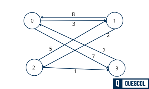
- Edge from 0 to 1 with weight 3
- Edge from 0 to 3 with weight 7
- Edge from 1 to 0 with weight 8
- Edge from 1 to 2 with weight 2
- Edge from 2 to 1 with weight 5
- Edge from 2 to 3 with weight 1
- Edge from 3 to 0 with weight 2
The graph’s adjacency matrix looks like this (using ∞ to represent no direct edge):
| From \ To | 0 | 1 | 2 | 3 |
|---|---|---|---|---|
| 0 | 0 | 3 | ∞ | 7 |
| 1 | 8 | 0 | 2 | ∞ |
| 2 | ∞ | 5 | 0 | 1 |
| 3 | 2 | ∞ | ∞ | 0 |
For Vertex 0 as intermediate (k = 0)
Given the current state of the matrix:
| From \ To | 0 | 1 | 2 | 3 |
|---|---|---|---|---|
| 0 | 0 | 3 | ∞ | 7 |
| 1 | 8 | 0 | 2 | ∞ |
| 2 | ∞ | 5 | 0 | 1 |
| 3 | 2 | ∞ | ∞ | 0 |
We update dist[i][j] = min(dist[i][j], dist[i][0] + dist[0][j]) for every (i, j).
Row i = 0
dist[0][0]: current 0, via 0 → 0 → 0 = 0 + 0 = 0 → min(0,0)=0 → no changedist[0][1]: current 3, via = 0 + 3 = 3 → no changedist[0][2]: current ∞, via = 0 + ∞ = ∞ → no changedist[0][3]: current 7, via = 0 + 7 = 7 → no change
Row i = 1
dist[1][0]: current 8, via = 8 + 0 = 8 → no changedist[1][1]: current 0, via = 8 + 3 = 11 → min(0,11)=0 → no changedist[1][2]: current 2, via = 8 + ∞ = ∞ → no changedist[1][3]: current ∞, via = 8 + 7 = 15 → min(∞,15)=15 → updatedist[1][3] = 15
Row i = 2
dist[2][0]: current ∞, via = ∞ + 0 = ∞ → no changedist[2][1]: current 5, via = ∞ + 3 = ∞ → no changedist[2][2]: current 0, via = ∞ + ∞ = ∞ → no changedist[2][3]: current 1, via = ∞ + 7 = ∞ → no change
Row i = 3
dist[3][0]: current 2, via = 2 + 0 = 2 → no changedist[3][1]: current ∞, via = 2 + 3 = 5 → min(∞,5)=5 → updatedist[3][1] = 5dist[3][2]: current ∞, via = 2 + ∞ = ∞ → no changedist[3][3]: current 0, via = 2 + 7 = 9 → min(0,9)=0 → no change
Updated Matrix after applying above operation
After applying these updates using k=1 as an intermediate vertex, the matrix becomes:
| From \ To | 0 | 1 | 2 | 3 |
|---|---|---|---|---|
| 0 | 0 | 3 | ∞ | 7 |
| 1 | 8 | 0 | 2 | 15 |
| 2 | ∞ | 5 | 0 | 1 |
| 3 | 2 | 5 | ∞ | 0 |
For Vertex 1 as intermediate (k = 1)
Given the current state of the matrix:
| From \ To | 0 | 1 | 2 | 3 |
|---|---|---|---|---|
| 0 | 0 | 3 | ∞ | 7 |
| 1 | 8 | 0 | 2 | 15 |
| 2 | ∞ | 5 | 0 | 1 |
| 3 | 2 | 5 | ∞ | 0 |
Now dist[i][j] = min(dist[i][j], dist[i][1] + dist[1][j]).
Row i = 0
dist[0][0]: current 0, via = 3 + 8 = 11 → min(0,11)=0 → no changedist[0][1]: current 3, via = 3 + 0 = 3 → no changedist[0][2]: current ∞, via = 3 + 2 = 5 → min(∞,5)=5 → updatedist[0][2] = 5dist[0][3]: current 7, via = 3 + 15 = 18 → min(7,18)=7 → no change
Row i = 1
dist[1][0]: current 8, via = 0 + 8 = 8 → no changedist[1][1]: current 0, via = 0 + 0 = 0 → no changedist[1][2]: current 2, via = 0 + 2 = 2 → no changedist[1][3]: current 15, via = 0 + 15 = 15 → no change
Row i = 2
dist[2][0]: current ∞, via = 5 + 8 = 13 → min(∞,13)=13 → updatedist[2][0] = 13dist[2][1]: current 5, via = 5 + 0 = 5 → no changedist[2][2]: current 0, via = 5 + 2 = 7 → min(0,7)=0 → no changedist[2][3]: current 1, via = 5 + 15 = 20 → min(1,20)=1 → no change
Row i = 3
dist[3][0]: current 2, via = 5 + 8 = 13 → min(2,13)=2 → no changedist[3][1]: current 5, via = 5 + 0 = 5 → no changedist[3][2]: current ∞, via = 5 + 2 = 7 → min(∞,7)=7 → updatedist[3][2] = 7dist[3][3]: current 0, via = 5 + 15 = 20 → min(0,20)=0 → no change
Updated Matrix after applying above operation
After applying these updates using k=1 as an intermediate vertex, the matrix becomes:
| From \ To | 0 | 1 | 2 | 3 |
|---|---|---|---|---|
| 0 | 0 | 3 | 5 | 7 |
| 1 | 8 | 0 | 2 | 15 |
| 2 | 13 | 5 | 0 | 1 |
| 3 | 2 | 5 | 7 | 0 |
For Vertex 2 as intermediate (k = 2)
Given the current state of the matrix:
| From \ To | 0 | 1 | 2 | 3 |
|---|---|---|---|---|
| 0 | 0 | 3 | 5 | 7 |
| 1 | 8 | 0 | 2 | 15 |
| 2 | 13 | 5 | 0 | 1 |
| 3 | 2 | 5 | 7 | 0 |
Now dist[i][j] = min(dist[i][j], dist[i][2] + dist[2][j]).
Row i = 0
dist[0][0]: current 0, via = 5 + 13 = 18 → min(0,18)=0 → no changedist[0][1]: current 3, via = 5 + 5 = 10 → min(3,10)=3 → no changedist[0][2]: current 5, via = 5 + 0 = 5 → no changedist[0][3]: current 7, via = 5 + 1 = 6 → min(7,6)=6 → updatedist[0][3] = 6
Row i = 1
dist[1][0]: current 8, via = 2 + 13 = 15 → min(8,15)=8 → no changedist[1][1]: current 0, via = 2 + 5 = 7 → min(0,7)=0 → no changedist[1][2]: current 2, via = 2 + 0 = 2 → no changedist[1][3]: current 15, via = 2 + 1 = 3 → min(15,3)=3 → updatedist[1][3] = 3
Row i = 2
dist[2][0]: current 13, via = 0 + 13 = 13 → no changedist[2][1]: current 5, via = 0 + 5 = 5 → no changedist[2][2]: current 0, via = 0 + 0 = 0 → no changedist[2][3]: current 1, via = 0 + 1 = 1 → no change
Row i = 3
dist[3][0]: current 2, via = 7 + 13 = 20 → min(2,20)=2 → no changedist[3][1]: current 5, via = 7 + 5 = 12 → min(5,12)=5 → no changedist[3][2]: current 7, via = 7 + 0 = 7 → no changedist[3][3]: current 0, via = 7 + 1 = 8 → min(0,8)=0 → no change
After applying these updates using k=2 as an intermediate vertex, the matrix becomes:
| From \ To | 0 | 1 | 2 | 3 |
|---|---|---|---|---|
| 0 | 0 | 3 | 5 | 6 |
| 1 | 8 | 0 | 2 | 3 |
| 2 | 13 | 5 | 0 | 1 |
| 3 | 2 | 5 | 7 | 0 |
For Vertex 3 as intermediate (k = 3)
Given the current state of the matrix:
| From \ To | 0 | 1 | 2 | 3 |
|---|---|---|---|---|
| 0 | 0 | 3 | 5 | 6 |
| 1 | 8 | 0 | 2 | 3 |
| 2 | 13 | 5 | 0 | 1 |
| 3 | 2 | 5 | 7 | 0 |
Now dist[i][j] = min(dist[i][j], dist[i][3] + dist[3][j]). (Start from matrix after k=2.)
Row i = 0
dist[0][0]: current 0, via = 6 + 2 = 8 → min(0,8)=0 → no changedist[0][1]: current 3, via = 6 + 5 = 11 → min(3,11)=3 → no changedist[0][2]: current 5, via = 6 + 7 = 13 → min(5,13)=5 → no changedist[0][3]: current 6, via = 6 + 0 = 6 → no change
Row i = 1
dist[1][0]: current 8, via = 3 + 2 = 5 → min(8,5)=5 → updatedist[1][0] = 5dist[1][1]: current 0, via = 3 + 5 = 8 → min(0,8)=0 → no changedist[1][2]: current 2, via = 3 + 7 = 10 → min(2,10)=2 → no changedist[1][3]: current 3, via = 3 + 0 = 3 → no change
Row i = 2
dist[2][0]: current 13, via = 1 + 2 = 3 → min(13,3)=3 → updatedist[2][0] = 3dist[2][1]: current 5, via = 1 + 5 = 6 → min(5,6)=5 → no changedist[2][2]: current 0, via = 1 + 7 = 8 → min(0,8)=0 → no changedist[2][3]: current 1, via = 1 + 0 = 1 → no change
Row i = 3
dist[3][0]: current 2, via = 0 + 2 = 2 → no changedist[3][1]: current 5, via = 0 + 5 = 5 → no changedist[3][2]: current 7, via = 0 + 7 = 7 → no changedist[3][3]: current 0, via = 0 + 0 = 0 → no change
After applying these updates using k=3 as an intermediate vertex, the matrix becomes:
| From \ To | 0 | 1 | 2 | 3 |
|---|---|---|---|---|
| 0 | 0 | 3 | 5 | 6 |
| 1 | 5 | 0 | 2 | 3 |
| 2 | 3 | 5 | 0 | 1 |
| 3 | 2 | 5 | 7 | 0 |
This matrix now represents the shortest path distances between all pairs of vertices when considering vertex 3 as an intermediate step in the paths. The value of dist[i][j] represents the shortest distance from vertex i to vertex j after incorporating paths that pass through vertex 3.
Real Life Applications
Floyd–Warshall is used in:
- GPS navigation systems (finding shortest routes between multiple locations).
- Airline route planning (shortest flight routes even with layovers).
- Network routing (finding quickest path for data packets between computers).
- Logistics (fastest delivery paths in a supply chain network).
Conclusion
The Floyd–Warshall algorithm is a fundamental method for solving the all-pairs shortest path problem in weighted graphs. It works by progressively considering each vertex as an intermediate point and updating the shortest distances between every pair of vertices. The algorithm is simple to implement, versatile enough to handle negative edge weights (excluding negative cycles), and ensures accurate shortest path computation.